IAEN Manual
IAEN: Graphical User Interface for Introduction to Ecological Network Analysis
Table of Contents
- 1 Introduction
- 2 Dependencies
- 3 Load the interface
- 4 Importing data
- 5 Metrics or Statistics
- 6 Presentation of graphics
- References
1 Introduction
In order to make the different R language routines accessible to all users for statistical analysis of networks and their graphs without the need for programming knowledge, a graphical user interface (GUI) was programmed. The IAEN package is a tool that provides a graphical user interface (GUI) which is implemented through the GTK+ toolkit implemented in the RGtk2 package and is stored in the GitHub repository. It allows you to manage data and use different types of tools for the analysis of ecological networks, as well as visualization and edition of graphics. There is a large repertoire of packages implemented in R that emphasize ecological network analysis for adjacent binary, weighted, and bipartite matrices. R also has a set of packages that allow to analyze and visualize different types of networks in general, each one has its different ways of managing databases.
Because of the aforementioned, this interface is made up of various packages stored in R that emphasize ecological networks and networks in general, allowing us to make use of functions easily and interactively without the user fully using the programming language of R. Basic and usual methods are used in which the package that is being used is specified in each process in order to spread the use of R and its packages, where if you want to do a more specific analysis you can consult the different functions included in the environment R. This document is intended to assist the user in the operation of the interface to make proper use of the different tools it provides. Each of the windows that comprise it is also described. In general, the user can import databases in the “File” tab, perform network analysis in the “Statistics” window, create binary networks and perform small world functions in the “Simulations” window and execute graphics in the “Graphs” window.
2 Dependencies
The list of dependencies that are required for the interface to run correctly is presented in Table 1, as well as the reason for which they were used. It is worth mentioning that there is a high dependence on enaR, cheddar and bipartite packages. This is because they are the packages that most emphasize the theme of ecological networks, in addition to containing functions of interest to our objective. Only some functions were implemented. Regarding graphics, some of these were done using the default functions of their package, while others were done using the ggplot2, gplots and ggraph packages to improve their resolution in some cases.
Table 1. List of required packages
| Paquetería | Descripción |
|---|---|
| RGtk2 (Lawrence and Temple, 2010) | Tools for creating graphical interfaces |
| cairoDevice (Lawrence, 2017) | |
| enaR (Lau et al., 2017) | Functions for ecological network analysis |
| cheddar (Hudson et al., 2018) | |
| bipartite (Dormann et al., 2008) | |
| readxl (Wickham and Bryan, 2018) | Data import and export |
| writexl (Ooms, 2018) | |
| network (Butts, 2015) | Functions for general network analysis |
| igraph (Csardi and Nepusz, 2006) | |
| sna (Butts, 2016) | |
| tnet (Opsahl, 2009) | |
| ggplot2 (Wickham, 2016) | Functions for editing and displaying graphics |
| ggraph (Pedersen, 2018) | |
| gplots (Warnes et al., 2016) | |
| scales (Wickham, 2017) | |
| reshape (Wickham, 2007) | Data restructuring |
| pryr (Wickham, 2018) | Create active links |
3 Load the Interface
Once the package installation process has been carried out and verified that it has been carried out successfully, the steps that follow are the following: firstly, you must load the package and then use the corresponding function to display the interface. The installation is only done once in each installed version of R or in the case of using R-Studio, as well as to load the package it is only done once in each open workspace, as shown below:
library(IAEN)
IAEN()
 |
 |
|---|---|
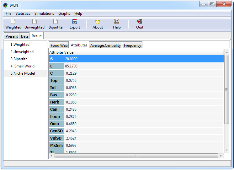 |
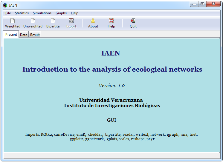
Figura 1. Interfaz gráfica de usuario
Figure 1 illustrates the interactive structure of the graphical interface when it has been loaded in the R-Studio console, where it can be seen that its component elements are a menu bar, a shortcut bar for quick import options, and data export, a set of tabs that includes a presentation, a tab called “Data” where you can view the data that has been loaded and a tab named “Result” where, through sub-tabs the different outputs of the analysis performed are shown. Different tabs grouped by type of functions are shown in the menu bar, such as the “File” tab that contains data import and export functions. The “Statistics” tab contains data analysis functions for the different types of networks (binary, weighted and bipartite). The “Simulation” tab shows a window with options to randomly create different types of food webs and perform functions used on small worlds. The “Graphs” tab shows a range of graphs that can be made for different types of networks. Finally, the “Help” tab provides general information on the package.
4 Importing data
- Adjacent matrix of a weighted network
Before loading a weighted matrix, the structure in which the data is required to be organized must be taken into account. This structure is based on the input arguments required in the enaR::pack function to create a network class object and in order to load and display it in the interactive interface, the following specifications are required:
– Equal adjacency matrix names for rows and columns, preferably non-numeric and without spaces.
– Contain numerical values.
– Avoid empty cells.
– Include a column specifying the living nodes (1) and the non-living nodes (0).
– Input, export, output, respiration, biomass and live vectors must be placed vertically to the adjacency matrix and in that order. – The column “Outputs” is the sum of respiration and exports, this vector is optional.
– The adjacent matrix, the vector of entries, exports and the vector of living items are mandatory, the others may or may not be considered. In case of not considering them, include a vector of zeros to avoid empty values.
–- The data should be ordered in the following way: the adjacent matrix is placed first, then the following columns the inputs (Inputs), exports (Exports), outputs (Outputs), respiration (Respiration), biomass (Biomass) and indicator of living (1) or not living (0) nodes (Living).
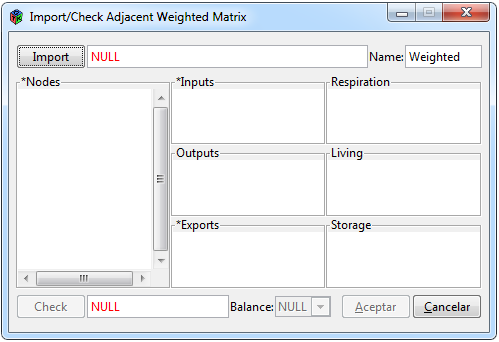
Figure 2. Window to import a weighted matrix
To be able to import a weighted matrix within the interface, you have to select the * Data> Import> Weighted tabs *, following these steps a window as in Figure 2 will appear, where the elements that make it up are a group of sections that have the purpose of showing that the loaded vectors are in the proper order. The functionality of the window is summarized in the following steps:
– Search for the file through the “Import” button, where you can choose files in Excel (.xls), Excel delimited by commas (.csv) or text (.txt) formats. – Name the new object, by default Weighted.
– The first vectors of the matrix will appear in the “Nodes” section.
– In automatic the rest of the vectors are accommodated in each of the sections.
– “Matrix”, “Input” and “Export” are mandatory, the other data are optional.
– Verify with the “Check” button that all the vectors are imported correctly, in case of being incorrect a pop-up window will be shown with the list of errors found, then check the data input format to correct the details.
– The balancing tab will be activated only if the matrix and the remaining vectors are not balanced, if it is the case, select the type of balancing that you want to execute, this function is taken from the enaR::balance function.
– Finally select the “Ok” button so that different objects are created and can be used when necessary, the data will be shown in the “Data” tab.
- Adjacent matrix of an unweighted network
Regarding the unweighted matrix, the specifications are different, among them it is highlighted that its structure is binary where the values that make it up must be numerical and only values with zeros and ones, where zero represents absence of predator-prey interaction and one when an interaction exists, must be included. Empty values should be avoided and row and column names should be included that should not have spaces and the matrix should be symmetric.
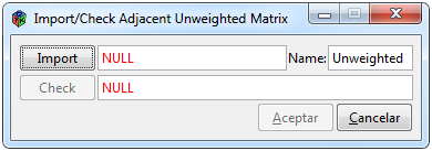
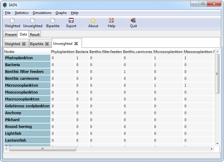
Figure 3. Window to import an unweighted matrix
To import an adjacent unweighted matrix or, in other words, a binary matrix, you must select the * Data> Import> Unweighted * tabs from the interface. Doing so a window like the one in Figure 3 will open. The “Import” button has the functionality of opening a window to search for the file to be imported, where the format to choose can be Excel (.xls), Comma delimited Excel (.csv) or text (.txt).
You can change the name of the matrix, by default Unweighted, this name will serve to name different objects that will be used in subsequent analyzes and to identify it within the interface. Once a file is selected, the “Check” button will be activated, which has the purpose of reviewing compliance with the aforementioned specifications., If it does not meet at least one of the restrictions, a pop-up window will appear to show the errors that have been found, if this is the case, the file must be reviewed and corrected.
- Adjacent matrix of a bipartite network
The steps to follow to import a bipartite matrix are very similar to those of a binary matrix, since the specifications are: include names of rows and columns preferably without spaces, avoid empty values and contain numerical values either binary (zeros and ones) or weighted. The only difference is that it can be of dimension pxq since this type of networks does not necessarily have to be symmetrical because they do not represent trophic interactions.
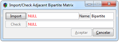
Figure 4. Window to import a bipartite matrix
On the other hand, to import an adjacent bipartite matrix, you must select the * Data> Import> Bipartite * tabs. The resulting window (Figure 4) is similar to that of an unweighted matrix, except that the default name is Bipartite and the specifications evaluated by the “Check” button are different. The “Import” button has the same functionality of showing a window to find the file you want to load with Excel (.xls), Excel delimited by commas (.csv) or text (.txt) options. By clicking on “Accept”, the necessary objects will be created to carry out the analyzes that are requested later and the data will be displayed on the interface in the “Data” tab.
5 Metrics or Statistics
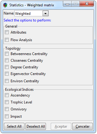
Figure 5. Statistics for a weighted network
To perform different statistics on a weighted network, select the * Statistics> Weighted * tabs, then the window shown in Figure 5 will appear. The Weighted tab will be activated only when an adjacent matrix of a weighted network has been imported into the interface. The window is divided into three sections, the “General” section that contains network metrics such as attributes and flow analysis, the “Topology” section that contains a set of different centralities and the “Ecological Indices” section that contains specific indicators for a trophic network. The “Name” tab shows the name of all the weighted networks that have been loaded in the interface, you have to select the network with which you want to carry out the analyzes.
Some attributes and the centralities of closeness, betweenness and degree were used using the tnet package, while the other centralities and other functions that emphasize ecological network analysis are performed using the enaR package. To know the description of each result, please see the documentation of the tnet (Opsahl, 2009) and enaR packages (Lau et al., 2017).
Finally, it contains a set of buttons to select and deselect all the categories included, and a button to accept and cancel the analysis. When clicking on accept, a loading icon will appear in the lower left of the interface in order to notify that some analyzes may require a long waiting time, the results will be displayed in the “Result” window through sub-tabs.
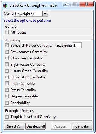
Figure 6. Statistics for an unweighted network
To perform different statistics for an unweighted network, select the * Statistics> Unweighted * tabs within the interface, it should be mentioned that this tab is only activated when an adjacent matrix of this type has been imported. The window is divided into three sections “General”, “Topology” and “Ecological Indices” (Figure 6). For the calculation of attributes the cheddar, igraph and network packages were used. In attributes, three simple functions were added, one that calculates the percentage of herbivorous species, another that shows the percentage of species that are included in loops or cycles, which was obtained by identifying the nodes included in the diagonal of the multiplication of the same matrix n times and finally the proportion of species that feed on prey of more than one trophic level.
In the “Topology” section, a group of centralities is shown as well as the reachability function. The centralities of betweenness, closeness and degree are calculated using the igraph package, while the others by using the sna package. The section of “Ecological Indices” contains the trophic level calculations and omnivory indicators. For this, the cheddar package was used. An omnivory indicator mentioned by Goldwasser and Roughgarden (1993) was included, which is based on the mean of the standard deviations of the chain lengths of each species to a basal species.
The “Name” tab shows all the binary matrices that have been loaded into the interface, from which one must be selected to perform the analyzes. To see the specifications of each result, please consult the documentation of igraph (Csardi and Nepusz, 2006), sna (Butts, 2016), cheddar (Hudson et al., 2018) and network (Butts, 2015). In the same way that the window of Figure 6 includes buttons to select and deselect the boxes and an accept and cancel button, in which clicking the accept button will include an icon in the lower left that indicates that the program is executing the corresponding algorithms and at the end the results will appear in sub-tabs in the “Result” section.
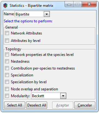
Figure 7. Statistics for a bipartite network
To perform statistics for a bipartite network, select the * Statistics> Bipartite * tabs, this tab will be activated only when an adjacent matrix of a bipartite network has been imported into the interface. Clicking on the previous tabs, a window like the one in Figure 7 will appear. The window is divided into two parts, the first contains general attributes of the network and the second called “Topology” contains more specific functions, both sections include functions of the bipartite package (Dormann et al., 2008), so to know the content of each indicator, please review the description of the functions in its documentation.
In the same way that in the windows of Figures 6 and 7, a “Name” tab is included to select the network with which you want to execute the functions, and buttons are included to select and deselect the boxes and a button to accept and cancel with the same functionalities.
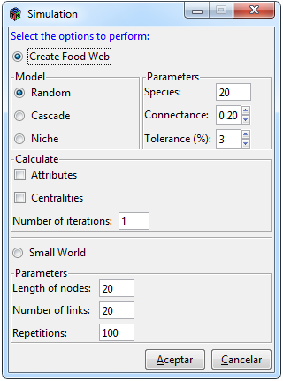
Figure 8. Simulation window
To carry out different simulation functions, you have to select the Simulations> Simulations tabs and thus visualize the window shown in Figure 8. The window contains two sections, one to create random food webs and another to execute functions used in small world networks. It has three methods to create food webs, the random model, the cascade model and the niche model, from which the attributes and centralities can be calculated, in turn this procedure can be performed n times and as a result a matrix will be obtained randomly and average attributes and centralities of the n repetitions, a matrix is also included with the number of times an interaction appeared at a specific position. Food web models have as argument the number of nodes or species, the value of connectivity on a scale of 0 to 1 and a value of percentage of tolerance that refers to the acceptance interval for connectivity, that is, in each simulation the function only includes networks that are in that interval of the parameter so that the parameter is consistent, as mentioned in Williams and Martinez (2000), by default 3%.
The random model (Williams and Martinez, 2000) is based on the Erdos and Rényi (1960) model, which consists of creating a network with n vertices representing the number of species (S), where all the links between species have the same probability P of existing equal to the connectivity (C) of the empirical network. In the cascade model (Cohen and Newman (1985); Williams and Martinez (2000)), each species has a probability P = 2CS / (S-1) of consuming another species with lower niche values. The model has a strict hierarchy of feeding since it prohibits the presence of cannibalism and cycles.
The niche model Williams and Martinez (2000) assigns to each species a niche value (ni) in the interval [0,1]. Each species feeds on the species that are in the range of niche values (ri) obtained from the beta distribution, which are placed using a value of center ci, allowing the presence of cannibalism and loops. The center ci of the feeding range ri is a uniform random number in the interval ri/2 and the minimum value between ni and 1-ri/2. To ensure that each network contains at least one basal species, the species with the smallest value has a rank value equal to zero. The algorithms of the three previously mentioned models were implemented in the graphical interface through their own algorithms, where functions are added that avoid the presence of nodes with double zeros and / or disconnected.
On the other hand, the second section includes the calculation of the characteristic path length (L) and the cluster coefficient (C), both parameters are used to test whether or not a network behaves like a small world (Watts and Strogatz, 1998). For the creation of the random graphs, the igraph::sample_gnm function was used, which generates graphs according to the Erdos-Rényi model, for the cluster coefficient the igraph::transitivity function was used and for the average length of the shortest path the igraph::mean_distance function, all three functions belong to the igraph package (Csardi and Nepusz, 2006). The required arguments in the graphical interface to obtain the L and C parameters are the number of nodes, the number of links and the number of repetitions that you want to perform to optimize the result. As a result, a table is obtained with the values of L and C of each of the repetitions as well as the average. Clicking on the accept button will display the results in the “Result” tab through sub-tabs either of food web creation or small world parameters.
Para realizar diferentes funciones de simulación se tienen que seleccionar las pestañas de Simulations> Simulations y así visualizar la ventana mostrada en la Figura 8. La ventana contiene dos secciones una para crear redes alimenticias aleatorias y otra para ejecutar funciones empleadas en redes de mundos pequeños. Posee tres métodos para crear redes alimenticias, el modelo aleatorio, el modelo de cascada y el modelo de nicho, de los cuales se puede calcular los atributos y centralidades, a su vez se puede realizar éste procedimiento n veces y como resultado se obtendrá una matriz aleatoria y el promedio de atributos y centralidades de las n repeticiones, también se incluye una matriz con el número de veces que una interacción apareció en una posición específica.
6 Presentation of graphics
Each graph contains a window with a section of options that contains different basic parameters that can be altered to carry them out, the most common being the font and node size, as well as the font and node color. Several graphs also have the argument of specifying whether you want to use the original name of the nodes or if you want to replace them with numbers and in some cases you can only use numbers to identify the node or only points, depending on the type of graph you want perform, this in order not to saturate the graph and to better appreciate the results. The number of parameters displayed in each window will depend on the type of graph you want to make. In addition, it contains a tab that shows the different networks that have been loaded in the interface, if you want to run a graph specifically of an unweighted network then only the names of that type of network will appear. Accept and cancel buttons are included at the bottom right of each window.
You can open a graph window by selecting the graph menu then the type of network and finally the type of graph to be made. Initially the tabs appear inactive, to activate it you have to import a network of the same type. The graphics menu contains the name of the original function of the package that was used in order for the user to be able to identify the corresponding function and know what procedure is being carried out. These packages have already been mentioned above. All the graphics windows have, on the upper left, a couple of buttons, a save button and an exit button, it also includes a tab to select the format in which you want to save, among the available formats are tiff, jpeg , png and eps.
 |
 |
|---|---|
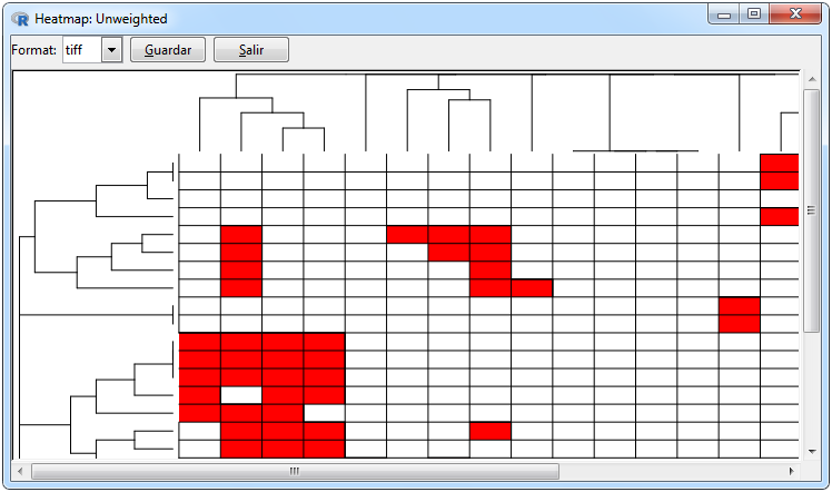 |
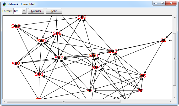
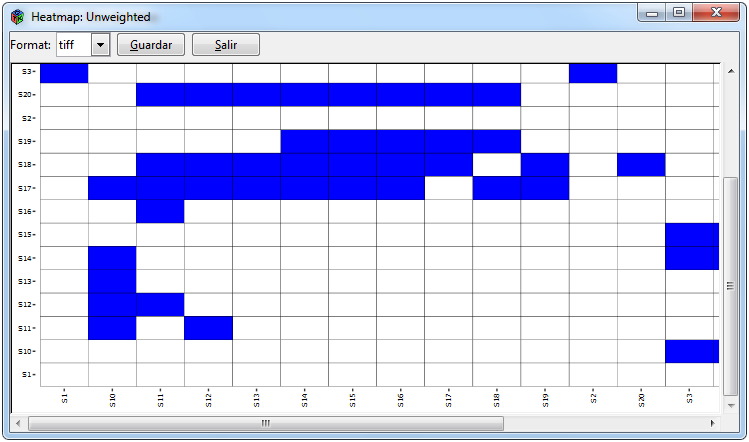
Figure 9: Graphics for any type of network
Figure 9 shows the graphs that can be made for any type of imported network. For the network, the ggraph package was used, which contains functions to graph networks through ggplot2, where if the matrix is bipartite, the nodes are ordered differently. The tabs to make a network is * Graph> Network> gplot. The other two graphs are heat maps that are intended to graphically represent the adjacent matrix in which the *Graph> Heat map> ggplot / heatmap.2 tabs must be selected in order to perform them.
One of the arguments to make a heat map is if you want to include cluster for rows and columns or not. In the first case of the heat map with a cluster, the headmap.2 function of the gplot package was used, also by default if the adjacent matrix is binary, it uses the Jaccard distance and the Ward method, while if the adjacent matrix is weighted, uses Euclidean distance and Ward’s method. In case you only want to graph the heatmap, the ggplot2 package is used.
 |
 |
|---|---|
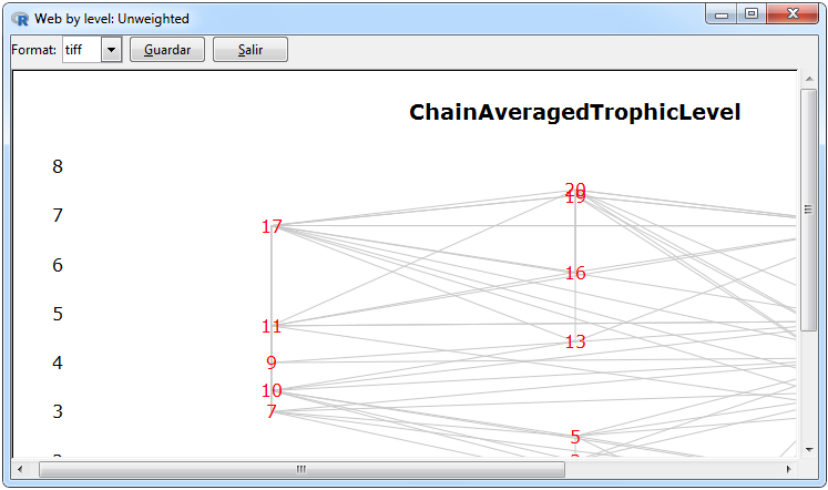 |
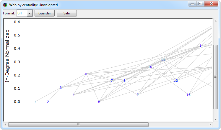
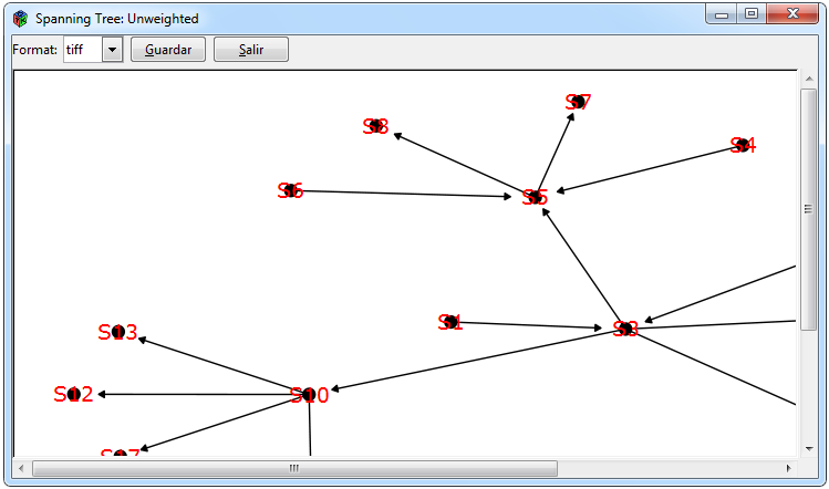
Figure 10. Graphics for an unweighted network
Figure 10 shows the graphs that can be made for a weighted network. The graphics of the ordered network with respect to some centrality and through the trophic levels were used through the default function of the cheddar package, one through the cheddar::PlotNPS function and the other through the cheddar::PlotWebByLevel function, the tabs to perform them are Graphs > Unweighted Matrix> Centrality> PlotNPS and * Graphs> Unweighted Matrix> Web By Level> PlotWeb- ByLevel * respectively. For the calculation of spanning tree the igraph::mst function of the igraph package was used and to graph it the igraph package using the * Graphs> Unweighted Matrix> Spanning Tree> mst * tabs.
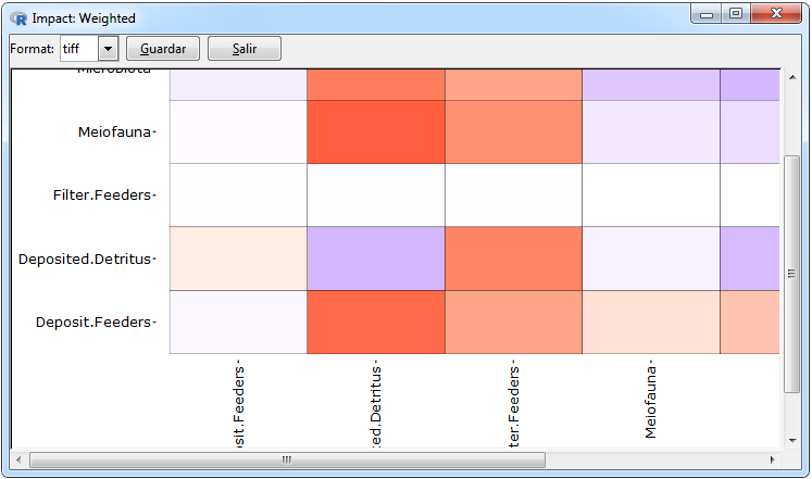
Figura 11. Impact graph for a weighted network
In the case of weighted networks, the only graph included in addition to the network and the heatmap to represent the adjacent matrix is a heat map made with functions from the ggplot2 package to represent the total trophic impacts of one species on another using the algorithm of Ulanowicz and Puccia (1990) implemented in the enaR package through the enaMTI function. The color for negative and positive values is included as an argument where if the values are close to zero, the corresponding color will degrade to white. An example of this type of graph is shown in Figure 11 where, in order to perform it, the following tabs Graph> Weighted> Impact> ggplot have to be followed.
 |
 |
|---|---|
 |
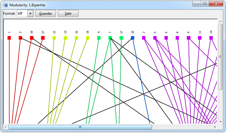 |
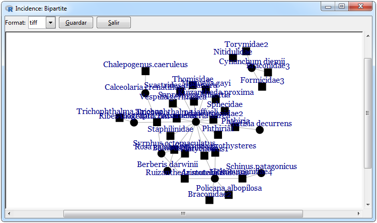
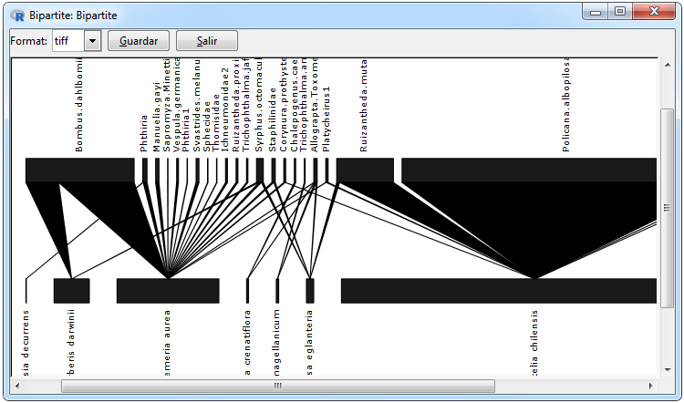
Figura 12. Graphics for a bipartite network
In Figure 12 the graphs that can be made for a bipartite network are shown, the first is an incidence network which makes a distinction through the figures for differences in the rows and columns of the adjacent matrix, this graph was used using the igraph package using the graph.incidence function and can be done using the Graphs> Bipartite Matrix> Network> graph.incidence tabs. The bipartite network was performed using the bipartite package since it is a clear way to visualize the weights in this type of network and can be done using the Graphs> Bipartite Matrix> Plot Web> plotweb tabs.
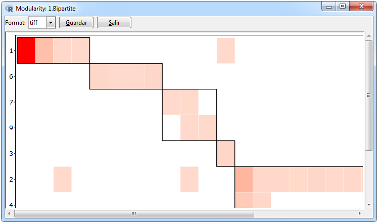
Two forms were used to visualize the modularity of the network, one through a heatmap where the clusters are differentiated through a grid and the other through a network with the nodes ordered with respect to the group to which they belong, in which for differences a group on the other a different color range was used., Both graphs were made using the ggplot2 package and can be done through the Graphs> Bipartite Matrix> Modularity> ggplot tabs. In the realization of a modularity graph, the calculation must first be done in the statistics window for a bipartite network which will use the bipartite::computeModules function. The graph window instead of showing a tab with the names of the imported bipartite networks will show the id of the modularity results that are in the results tab.
References
Butts, C.T. (2015). network: Classes for Relational Data. R package version 1.13.0.1. The Statnet Project (http://statnet.org). url: http://CRAN.R-project.org/package=network.
Butts, C.T. (2016). sna: Tools for Social Network Analysis. R package version 2.4. url: https://CRAN.R-project.org/package=sna.
Cohen, J.E. and C.M. Newman (1985). “A stochastic theory of community food webs I. Models and aggregated data”. In: Proc. R. Soc. Lond. B 224.1237, pp. 421-448.
Csardi, G. and T. Nepusz (2006). “The igraph software package for complex network research”. In: InterJournal Complex Systems, p. 1695. url: http://igraph.org.
Dormann, C.F., B. Gruber, and J. Fruend (2008). “Introducing the bipartite Package: Analysing Ecological Networks”. In: R News 8.2, pp. 8-11.
Erdos, P. and A. Renyi (1960). “On the evolution of random graphs”. In: Publ. Math. Inst. Hung. Acad. Sci 5.1, pp. 17-60.
Goldwasser, L. and J. Roughgarden (1993). “Construction and analysis of a large Caribbean food web”. In: Ecology 74.4, pp. 1216-1233.
GTK+ (2007). The Gimp Tool Kit. url: http://www.gtk.org/.
Hudson, L., D. Reuman, and R. Emerson (2018). Cheddar: analysis and visualization of ecological communities. R package version 0.1-633. url: https://github.com/quicklizard99/cheddar/.
Lau, M.K. et al. (2017). enaR: Tools for Ecological Network Analysis. R package version 3.0.0. url: https://CRAN.R-project.org/package=enaR.
Lawrence, M. (2017). cairoDevice: Embeddable Cairo Graphics Device Driver. R package version 2.24. url: https://CRAN.R-project.org/package=cairoDevice.
Lawrence, M. and D. Temple (2010). “RGtk2: A Graphical User Interface Toolkit for R”. In: Journal of Statistical Software 37.8, pp. 1-52. url: http://www.jstatsoft.org/v37/i08/.
Makiyama, K. (2018). githubinstall: A Helpful Way to Install R Packages Hosted on GitHub. R package version 0.2.2. url: https://CRAN.R-project.org/package=githubinstall.
Ooms, J. (2018). writexl: Export Data Frames to Excel ‘xlsx’ Format. R package version 1.0. url: https://CRAN.R-project.org/package=writexl.
Opsahl, T. (2009). Structure and Evolution of Weighted Networks. University of London (Queen Mary College), London, UK, pp. 104-122. url: http://toreopsahl.com/publications/thesis/.
Pedersen, T.L. (2018). ggraph: An Implementation of Grammar of Graphics for Graphs and Networks. R package version 1.0.2. https://CRAN.R-project.org/package=ggraph.
Ulanowicz, R.E. and C.J. Puccia (1990). “Mixed trophic impacts in ecosystems”. In: Coenoses, pp. 7{16.
Warnes, G.R. et al. (2016). gplots: Various R Programming Tools for Plotting Data. R package version 3.0.1. url: https://CRAN.R-project.org/package=gplots.
Watts, D.J. and S.H. Strogatz (1998). “Collective dynamics of `small-world’networks”. In: nature 393.6684, p. 440.
Wickham, H. (2007). “Reshaping data with the reshape package”. In: Journal of Statistical Software 21.12. url: http://www.jstatsoft.org/v21/i12/paper.
Wickham, H. (2016). ggplot2: Elegant Graphics for Data Analysis. Springer-Verlag New York. isbn: 978-3-319-24277-4. url: http://ggplot2.org.
Wickham, H. (2017). scales: Scale Functions for Visualization. R package version 0.5.0. url: https://CRAN.R-project.org/package=scales.
Wickham, H. (2018). pryr: Tools for Computing on the Language. R package version 0.1.4. url: https://CRAN.R-project.org/package=pryr.
Wickham, H. and J. Bryan (2018). readxl: Read Excel Files. R package version 1.1.0. url: https://CRAN.R-project.org/package=readxl.
Wickham, H., J. Hester, and W. Chang (2018). devtools: Tools to Make Developing R Packages Easier. R package version 1.13.6. url: https://CRAN.R-project.org/package=devtools.
Williams, R.J. and N.D. Martinez (2000). “Simple rules yield complex food webs”. In: Nature 404.6774, p. 180.